Understanding Laplace Transforms for Solving Differential Equations of Dynamic Systems
The video introduces the Laplace transform as a powerful tool for analyzing dynamic systems, using the example of a forced harmonic oscillator, where initial irregular motion transitions to a consistent rhythm.

Opening Puzzle [0:00]
The video begins by presenting a simulation of a mass on a spring influenced by an oscillating external force. Initially, the system exhibits irregular behavior before settling into a consistent rhythm. The central questions posed are:
- How can this irregular startup trajectory be mathematically analyzed?
- How long does it take for the system to reach its steady rhythm?
- What determines the amplitude of the oscillations once it stabilizes?
The Laplace transform is introduced as a powerful tool to study such dynamic systems and differential equations.
Simulation of a mass on a spring with an oscillating external force, showing initial irregular motion transitioning to a regular pattern over time. [ 00:00:30 ]
Key Properties of a Laplace Transform [1:06]
This section recaps fundamental concepts from previous chapters on Laplace transforms:
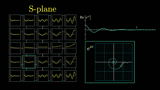
- S-plane and
e^stfunctions: The s-plane is a complex plane representing values of 's' ine^st.- Larger imaginary values of 's' correspond to more oscillation.
- Negative real parts of 's' indicate decay, while positive real parts indicate growth.
- Many natural functions can be decomposed into exponential pieces.
The S-plane mapping complex values of 's' to the behavior of e^st, showing how different regions correspond to oscillation, decay, or growth in the real part of the exponential function. [ 00:01:40 ]
- Laplace Transform Definition: The transform converts a time-domain function
f(t)into an s-domain functionF(s).- Poles in the
F(s)plot correspond to the exponential pieces hidden withinf(t).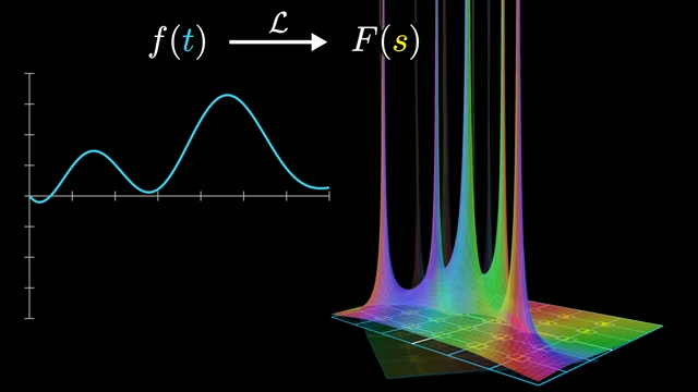
A function f(t) is transformed into F(s), where poles in the s-plane representation of F(s) reveal the exponential components of f(t). [ 00:02:30 ]
- Poles in the
- Property 1: Exponential to Fraction:
L{e^at} = 1/(s-a).- This means an exponential function in the time domain corresponds to a pole in the s-plane at value
a.
The Laplace transform of e^(at) is 1/(s-a), which is visualized as a pole at 'a' in the s-plane. [ 00:02:50 ]
- This means an exponential function in the time domain corresponds to a pole in the s-plane at value
- Property 2: Linearity:
L{a*f(t) + b*g(t)} = a*F(s) + b*G(s).- A scaled sum of functions transforms into the same scaled sum of their individual transforms.
- This implies that a function expressible as a sum of exponentials will transform into a sum of fractions, with each fraction having a pole corresponding to an exponential piece.

The linearity property of the Laplace transform, showing that the transform of a scaled sum of functions is the scaled sum of their individual transforms, leading to multiple poles in the s-domain for a sum of exponentials. [ 00:03:30 ]
Qualitative Analysis with Laplace Transforms [3:29]
The properties of Laplace transforms enable qualitative analysis of a system's dynamics:
- Imaginary poles: Indicate oscillation in the system.
- Negative real parts of poles: Suggest a tendency for the system to decay towards zero (stability).
- Positive real parts of poles: Point to instability, where the system tends to explode away from zero (growth).

Visual representation of how the location of poles in the s-plane (imaginary part for oscillation, real part for decay/growth) informs the qualitative behavior of a system's time-domain function. [ 00:04:00 ]
The Laplace Transforms of a Derivative [4:29]
A third crucial property allows for the transformation of differential equations into algebraic ones:
- Property 3:
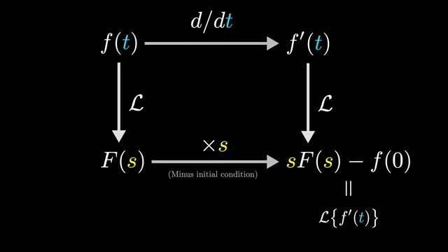
L{f'(t)} = sF(s) - f[<a href="https://youtube.com/watch?v=FE-hM1kRK4Y&t=0">0</a>].- This transforms differentiation in the time domain (
d/dt) into multiplication bysin the s-domain. - The
f[<a href="https://youtube.com/watch?v=FE-hM1kRK4Y&t=0">0</a>]term represents the initial condition, which is automatically incorporated into the transformed equation.
A diagram showing that the Laplace transform of a derivative, L{f'(t)}, is equivalent to multiplying the Laplace transform of f(t), F(s), by s and subtracting the initial condition f[<a href="https://youtube.com/watch?v=FE-hM1kRK4Y&t=0">0</a>]. [ 00:05:09 ]
- This transforms differentiation in the time domain (
The Forced Oscillator [6:06]
The video demonstrates applying Laplace transforms to solve the forced harmonic oscillator problem:
- System Description: A mass on a spring with damping is subjected to an external oscillating force
F0 cos(ωt).- The differential equation is
mx''(t) + μx'(t) + kx(t) = F0 cos(ωt).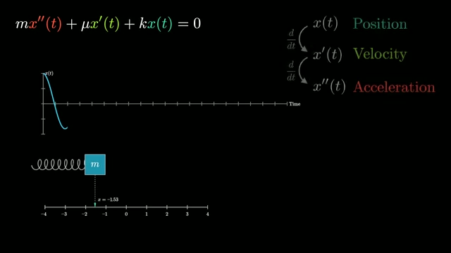
The differential equation for an unforced, damped harmonic oscillator, mx''(t) + μx'(t) + kx(t) = 0, along with a visual representation of the mass-spring system. [ 00:06:52 ] 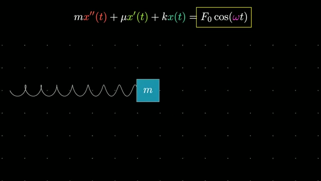
The differential equation mx''(t) + μx'(t) + kx(t) = F0 cos(ωt) representing a mass on a spring with damping and an external oscillating force. [ 00:07:19 ]
- The differential equation is
- General Strategy:
- Take the Laplace transform of all terms in the differential equation.
- Solve the resulting algebraic equation to find the transformed solution
X(s). - Invert the Laplace transform to recover the solution
x(t)in the time domain.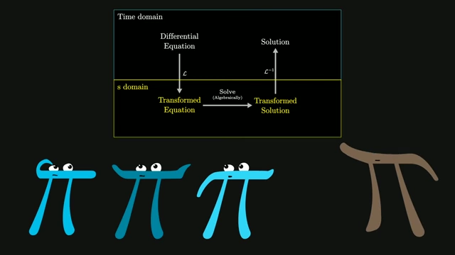
A flowchart illustrating the general strategy for solving differential equations using Laplace transforms: transform to s-domain, solve algebraically, then invert back to time domain. [ 00:08:19 ]
- Transforming the Equation:
L{x(t)} = X(s)L{x'(t)} = sX(s) - x0(wherex0is initial position)L{x''(t)} = s^2 X(s) - sx0 - v0(wherev0is initial velocity)- For simplicity, assume
x0 = 0andv0 = 0. - The left side
m x''(t) + μx'(t) + kx(t)transforms intoX(s)(ms^2 + μs + k). - The right side
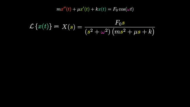
F0 cos(ωt)transforms intoF0s / (s^2 + ω^2). - Combining these yields the transformed solution:
L{x(t)} = X(s) = (F0s) / ((s^2 + ω^2)(ms^2 + μs + k)).
The final Laplace transformed solution X(s) for the forced harmonic oscillator, showing the driving force and system impedance terms in the denominator. [ 00:11:58 ]
Intuition from the Transformed Solution [11:59]
Analyzing the poles of the transformed solution X(s) provides insight into the system's behavior:
- Poles from
(ms^2 + μs + k) = 0: These roots typically have negative real parts and imaginary parts (assuming damping and oscillation).- They represent the natural resonant frequency of the unforced oscillator, indicating a decaying oscillation.
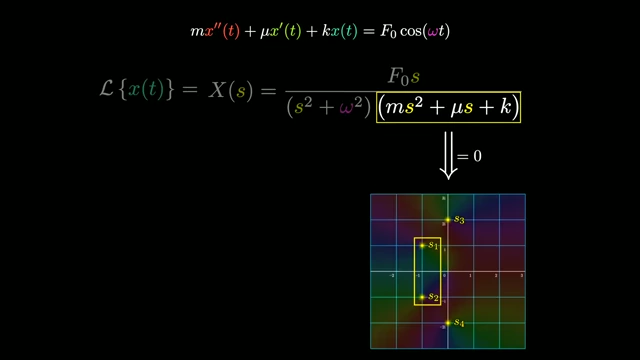
The poles in the s-plane originating from the system's natural dynamics (ms^2 + μs + k = 0) are shown, which correspond to decaying oscillations. [ 00:12:38 ]
- They represent the natural resonant frequency of the unforced oscillator, indicating a decaying oscillation.
- Poles from
(s^2 + ω^2) = 0(i.e.,s = ±iω): These are pure imaginary poles.- They correspond to the frequency of the external cosine force, representing a pure, undamped oscillation.

The poles on the imaginary axis (s = ±iω) arising from the external cosine forcing function, indicating sustained oscillation at the forcing frequency. [ 00:13:28 ]
- They correspond to the frequency of the external cosine force, representing a pure, undamped oscillation.
- Combined Dynamics: The total solution
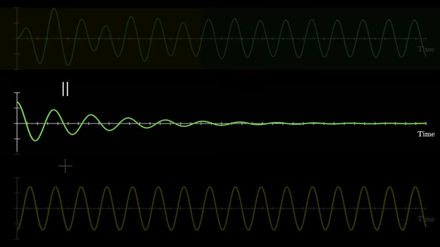
x(t)is a sum of components corresponding to these poles.- The decaying oscillation from the system's natural frequency (transient response) combined with the pure oscillation from the external force (steady-state response).
The total solution is decomposed into two components: the decaying oscillation from the unforced system and the sustained oscillation from the external driving force. [ 00:14:27 ] 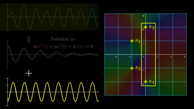
The s-plane poles (natural and forced) corresponding to the two components of the time-domain solution: a decaying oscillation and a sustained oscillation. [ 00:14:46 ] - This explains the initial "wibbling" period in the simulation, where both frequencies interact, eventually settling into the steady-state rhythm driven by the external force as the natural oscillation decays.
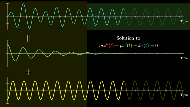
Illustration of how the initial "wibbling" behavior of the forced oscillator results from the superposition of the decaying natural oscillation and the steady-state driven oscillation, with the natural oscillation eventually fading away. [ 00:15:07 ]
- The decaying oscillation from the system's natural frequency (transient response) combined with the pure oscillation from the external force (steady-state response).
Inverting to Find a Final Answer [15:15]
To obtain the exact time-domain solution x(t), the inverse Laplace transform is applied:
- Partial Fraction Decomposition: The transformed solution
X(s)is broken down into a sum of simpler fractions, each corresponding to one of its poles (roots of the denominator).- Example:
X(s) = c1/(s-r1) + c2/(s-r2) + c3/(s-r3) + c4/(s-r4). - Solving for the constants (c_n) is required.

The process of partial fraction decomposition is shown, breaking down X(s) into a sum of simpler fractions, each with a denominator based on one of the roots (poles) of the original denominator. [ 00:15:47 ] 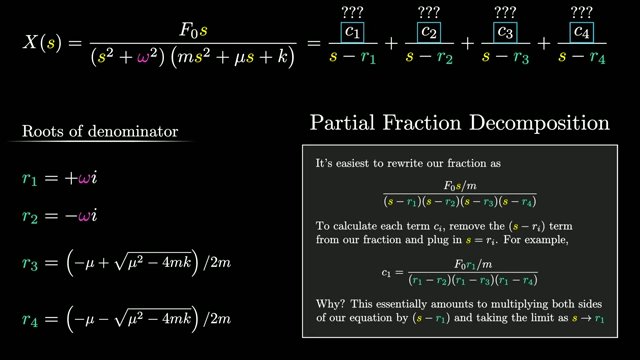
Detailed steps for calculating the constants (c_n) in partial fraction decomposition, demonstrating how to rewrite the fraction and solve for c1. [ 00:16:01 ]
- Example:
- Inverse Transform of Each Term: Each simple fraction
c_n/(s-r_n)inverts back into an exponential termc_n * e^(r_n * t). - Steady-State Amplitude: Focusing on the poles
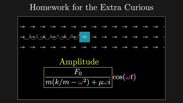
±iω(from the external force), their corresponding terms combine to form the steady-state cosine rhythm:(F0 / (m(k/m - ω^2) + 2μiω)) * 2cos(ωt).- The homework exercise is to analyze how the amplitude of this final expression depends on the difference between the resonant frequency of the spring and the frequency of the external force (
k/m - ω^2), which relates to phenomena like resonance in bridges.
The amplitude component of the final steady-state cosine oscillation, derived from the inverse Laplace transform, is highlighted, prompting consideration of its dependence on the difference between the resonant and forcing frequencies. [ 00:17:17 ]
- The homework exercise is to analyze how the amplitude of this final expression depends on the difference between the resonant frequency of the spring and the frequency of the external force (
Explaining the Derivative Property [17:40]
The video provides three ways to understand why L{f'(t)} = sF(s) - f[<a href="https://youtube.com/watch?v=FE-hM1kRK4Y&t=0">0</a>] is true:
- 1. Elementary but Limited (Testing an Example) [18:10]:
- Demonstrates that for
f(t) = e^at, applying the derivative and then the Laplace transform yieldsa/(s-a). - Algebraically manipulating
sF(s) - f[<a href="https://youtube.com/watch?v=FE-hM1kRK4Y&t=0">0</a>]for this function also results ina/(s-a), proving consistency for this specific case. - This approach provides intuition but is not a general proof; however, it can be extended to combinations of exponentials due to linearity.
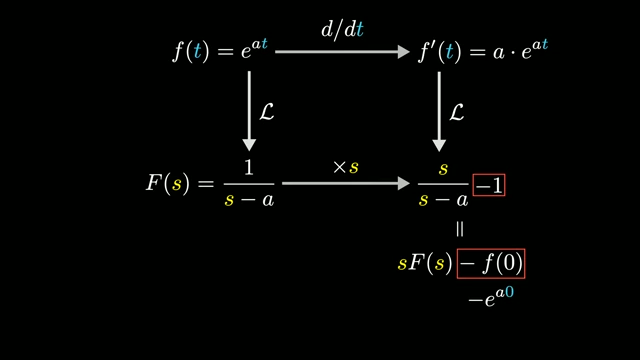
Testing the derivative property with f(t) = e^(at), showing that both paths (differentiate then transform, or transform then multiply by s and subtract initial condition) lead to the same result. [ 00:19:36 ]
- Demonstrates that for
- 2. General but Opaque (Integration by Parts) [20:25]:
- The formal derivation uses the definition of the Laplace transform as an integral (
L{f'(t)} = ∫[0,∞] f'(t)e^(-st) dt) and applies integration by parts. - This method rigorously proves the property but can obscure the underlying intuition.
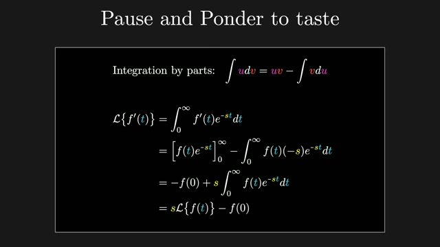
The derivation of the Laplace transform of a derivative using integration by parts, a formal but less intuitive method. [ 00:20:46 ]
- The formal derivation uses the definition of the Laplace transform as an integral (
- 3. Favorite but Theoretical (Reinventing the Transform) [21:13]:
- This explanation, to be covered in the next chapter, involves understanding the inverse Laplace transform and contour integrals.
- The idea is to logically "reinvent" the Laplace transform and its inverse from the goal of converting derivatives into multiplication, showing the property is inherent to the transform's design. This connects to Fourier series and transforms.
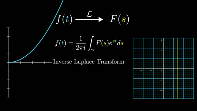
The mathematical formula for the inverse Laplace transform is introduced as a concept for future discussion, hinting at how its understanding can provide a deeper intuition for the derivative property. [ 00:21:26 ]