Implementing an MLP Character-Level Language Model with Core Machine Learning Concepts (Makemore Part 2)
This video demonstrates building a Multi-Layer Perceptron (MLP) character-level language model, expanding on the previous bigram model. It addresses the limitation of exponential growth in context by introducing word embeddings, where characters are mapped to lower-dimensional feature vectors. The process involves:
- Setting up the training dataset with a
block_sizeto define context length. - Implementing an embedding lookup table and understanding PyTorch tensor
viewoperations for efficient data handling. - Constructing the hidden layer with
tanhnon-linearity and an output layer to predict the next character. - Calculating the negative log likelihood loss, transitioning to PyTorch's efficient and numerically stable
F.cross_entropyfunction. - Developing a training loop using mini-batches for faster, approximate gradient updates.
- Strategies for finding an optimal learning rate by plotting loss against exponentially spaced learning rate exponents.
- Splitting the dataset into train, validation, and test sets to prevent overfitting and evaluate model generalization.
- Experiments with increasing hidden layer size and embedding dimensionality, showing how these hyperparameters affect performance.
- Visualizing 2D character embeddings, revealing interesting clusters (e.g., vowels together).
- Finally, the model is used to sample new, more "name-like" words, showcasing improved language generation compared to the bigram model.

MLP Language Model Architecture [ 00:05:50 ]
Introduction and Motivation [00:00:00]
The video continues the "makemore" series, moving from simple bigram models to a more advanced neural network. The previous bigram model used only a single preceding character, leading to poor name generation and an exponential increase in table size when considering longer contexts.

Bengio et al. 2003 (MLP Language Model) Paper Walkthrough [00:01:48]
The new approach is based on the influential Bengio et al. [2003] paper, "A Neural Probabilistic Language Model," which introduced using neural networks for language modeling.
- Addressing the curse of dimensionality: The paper proposes associating each word with a lower-dimensional feature vector, or "embedding," (e.g., 30 dimensions for a vocabulary of 17,000 words).
- These embeddings are initialized randomly but are tuned during training via backpropagation.
- Words with similar meanings or contexts are expected to cluster together in this embedding space, enabling generalization to unseen phrases.
- Neural Network Architecture:
- The model takes N previous words (or characters in this video's implementation) as input.
- Each input word index is looked up in an embedding table (C) to get its feature vector.
- These embeddings are concatenated to form the input to a hidden layer.
- The hidden layer applies a
tanhnon-linearity. - An output layer then projects the hidden state to a vector of logits, representing scores for each possible next word/character.
- A
softmaxfunction converts these logits into a probability distribution over the next word/character. - The model is trained by maximizing the log-likelihood of the correct next word/character.
Neural Network Architecture for a Language Model [ 00:05:50 ] - The
Cmatrix and the weights and biases of the hidden and output layers are the parameters optimized by backpropagation.
- The
(Re-)building Our Training Dataset [00:09:03]
The dataset consists of a list of names.
- Vocabulary and Mappings:
- Create a mapping from characters (strings) to integers and vice-versa, including a special '.' token for start/end of words.
- Context Length (
block_size):- Defined as the number of previous characters used to predict the next. For this video, it's initially set to 3.
- Generating (Context, Target) Pairs:
- For each word in the dataset, a rolling window approach is used.
- Example: For "emma" and
block_size=3:- Context:
..., Target:e - Context:
..e, Target:m - Context:
.em, Target:m - Context:
emm, Target:a - Context:
mma, Target:.
- Context:
- These pairs form the input
X(context as integer indices) and targetY(next character's integer index).
Code snippet showing character-to-integer mappings and dataset creation for the character-level language model. [ 00:09:30 ] - Initially, a small subset (e.g., first 5 words) is used to quickly develop the code. The full dataset contains over 228,000 examples.

First few examples of (context, target) pairs (X, Y) from the "emma" word. [ 00:10:30 ]
Implementing the Embedding Lookup Table [00:12:19]
- Embedding Matrix
C:- A
torch.randntensor is initialized with dimensions(vocab_size, embedding_dim). - Initially,
embedding_dimis set to 2 to allow for visualization. For 27 possible characters,Cis a 27x2 matrix.
- A
- Indexing
C:- PyTorch allows direct indexing of
Cusing integer tensors for efficiency. C[X]whereXis a(num_examples, block_size)tensor of integers, will directly return a(num_examples, block_size, embedding_dim)tensor of embeddings.- This is computationally equivalent to a one-hot encoding followed by matrix multiplication, but much faster.
- PyTorch allows direct indexing of
Implementing the Hidden Layer + Internals of torch.Tensor: Storage, Views [00:18:35]
- Weights and Biases:
W1(weights) is(input_dim, hidden_layer_size), andB1(biases) is(hidden_layer_size).- The
input_dimfor the hidden layer isblock_size * embedding_dim(e.g., 3 * 2 = 6 initially). hidden_layer_sizeis a hyperparameter, initially 100.
- Reshaping Embeddings:
- The
(num_examples, block_size, embedding_dim)embeddings need to be reshaped to(num_examples, block_size * embedding_dim)for matrix multiplication withW1. - This is achieved efficiently using
embeddings.view(-1, block_size * embedding_dim). torch.TensorInternals (Storage and Views):view()creates a new logical interpretation of the same underlying physical memory (storage) without copying data. This is very efficient.torch.cat()(concatenate) creates new memory to store the concatenated tensor, making it less efficient for reshaping operations whenviewis possible.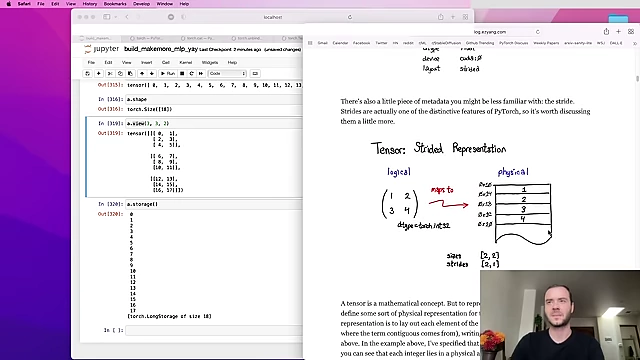
Diagram illustrating how a tensor's physical storage (1D) can be logically interpreted in different shapes (views) without data copying. [ 00:25:30 ]
- The
- Hidden State Calculation:
h = torch.tanh(embeddings_reshaped @ W1 + B1).- Biases (
B1) are automatically broadcasted across thenum_examplesdimension.
Code block showing the initialization of the hidden layer, embedding transformation, and the hidden state calculation. [ 00:28:00 ]
Implementing the Output Layer [00:29:15]
- Weights and Biases:
W2(weights) is(hidden_layer_size, vocab_size), andB2(biases) is(vocab_size).- The
vocab_sizeis 27 (for 26 letters + '.').
- Logits Calculation:
logits = h @ W2 + B2. These are the raw scores before probability normalization.
Implementing the Negative Log Likelihood Loss [00:29:53]
- Manual Loss Calculation Steps:
counts = logits.exp(): Exponentiate logits to get "fake counts" (non-normalized probabilities).probs = counts / counts.sum(1, keepdim=True): Normalize counts across rows to get probabilities summing to 1.loss = -probs[range(num_examples), Y].log().mean(): Select the probability assigned to the true target character for each example, take its log, negate, and then average.
Code block showing the manual calculation of probabilities from logits and then the negative log likelihood loss. [ 00:30:00 ]
Summary of the Full Network [00:32:17]
All parameters (embedding table C, W1, B1, W2, B2) are defined. The initial loss (before training) is around 17, indicating random predictions.

Introducing F.cross_entropy and Why [00:32:49]
PyTorch's torch.nn.functional.cross_entropy function should be used in practice for classification loss.
- Benefits:
- Efficiency: It internally fuses multiple operations into optimized kernels, avoiding the creation of intermediate tensors and reducing memory overhead.
- Simplified Backward Pass: The analytical derivative of cross-entropy is often simpler and more efficient to compute than chaining individual derivatives.
- Numerical Stability: It handles extreme logit values gracefully.
- Large positive logits can cause
exp()to overflow (resulting ininfthenNaN). F.cross_entropysubtracts the maximum logit from all logits before exponentiation. This "shifting" doesn't change the final probabilities (due to softmax properties) but brings numbers into a safer range (max logit becomes 0, others become negative), preventing overflow.
Example of numerical instability when logits are too large, leading to NaN values, and how `F.cross_entropy` addresses it. [ 00:36:00 ]
Implementing the Training Loop, Overfitting One Batch [00:37:56]
- Training Steps:
- Set all parameter gradients to zero (
p.grad.zero_()). - Perform a forward pass to calculate the loss (
loss = F.cross_entropy(logits, Y)). - Perform a backward pass (
loss.backward()) to compute gradients for all parameters. - Update parameters (
p.data -= learning_rate * p.grad).
- Set all parameter gradients to zero (
- Overfitting a Small Batch:
- Initially, the model is trained on a small subset (e.g., 32 examples).
- With 3,400 parameters, the model quickly achieves a very low loss (e.g., 0.05), demonstrating its capacity to memorize the data.
- The loss doesn't reach exactly zero if multiple target characters are associated with the same context in the dataset (e.g.,
...can predict 'e', 'o', 'a', 's').
Training loop code snippet showing gradient zeroing, backward pass, and parameter update. [ 00:38:30 ]
Training on the Full Dataset, Minibatches [00:41:25]
- Full Dataset:
- The full dataset has over 228,000 examples. Processing all of them in one go (
full-batch gradient descent) is computationally expensive and slow.
- The full dataset has over 228,000 examples. Processing all of them in one go (
- Mini-batch Gradient Descent:
- In practice,
mini-batchesof data are randomly sampled for each training step. - This provides an approximate gradient direction but allows for many more updates in the same amount of time, leading to faster overall convergence.
- Example: Select 32 random indices (
ix = torch.randint(...)) and useX[ix]andY[ix]for training.
Code block showing how to implement mini-batching by randomly selecting indices from the full dataset. [ 00:43:10 ] 
Benefit of mini-batching: approximate gradients allow more frequent updates, leading to faster training despite less precise gradient direction. [ 00:44:20 ]
- In practice,
Finding a Good Initial Learning Rate [00:45:40]
- Learning Rate Tuning:
- The learning rate (
lr) is a crucial hyperparameter. Too small, and training is slow; too large, and the loss might diverge (explode). - A common strategy is to sweep through learning rates and plot their effect on the loss.
- The learning rate (
- Exponentially Spaced Learning Rates:
- It's often more effective to search for
lron a logarithmic scale. - Create a range of learning rate exponents (e.g.,
lre = torch.linspace(-3, 0, 1000)for10^-3to10^0). - The actual learning rates are then
10**lre. - Train the model for a few steps with each
lrand record the loss.
- It's often more effective to search for
- Visualization:
- Plotting
lreagainst loss often reveals a "valley" where the loss decreases steadily before becoming unstable. The bottom of this valley suggests a good learning rate (e.g.,10^-1 = 0.1).
Plot of learning rate exponent versus loss, showing a "valley" indicating optimal learning rates. [ 00:50:40 ]
- Plotting
- Training with Chosen LR:
- Start with the identified optimal learning rate (e.g., 0.1) for many iterations.
- Periodically,
decaythe learning rate (e.g., multiply by 0.1) in later stages of training to fine-tune the model and prevent oscillations around the minimum.
Splitting Up the Dataset into Train/Val/Test Splits and Why [00:53:20]
- The Problem of Overfitting:
- A very powerful model might achieve a very low loss on the training data by simply memorizing it (
overfitting), without learning generalizable patterns. - Such a model performs poorly on unseen data and might only generate data identical to its training set.
- A very powerful model might achieve a very low loss on the training data by simply memorizing it (
- Solution: Data Splits:
- Training Set (e.g., 80%): Used exclusively for optimizing the model's parameters (weights, biases, embeddings) via gradient descent.
- Development/Validation Set (e.g., 10%): Used for tuning hyperparameters (e.g., hidden layer size, embedding dimension, learning rate schedule, regularization strength). The best model configurations are chosen based on their performance on this set.
- Test Set (e.g., 10%): Used only once at the very end to provide a final, unbiased estimate of the model's performance on completely unseen data. Repeated evaluation on the test set can lead to "overfitting" the test set itself.

Diagram illustrating the typical 80/10/10 split of a dataset into training, development (validation), and test sets. [ 00:54:40 ]
- Implementation:
- The full dataset of words is shuffled and then split into three partitions (
X_train,Y_train), (X_dev,Y_dev), and (X_test,Y_test). - Initial training with a small model (100 hidden neurons, 2D embeddings) shows similar train and dev loss (e.g., 2.3 vs 2.38), indicating
underfitting(model not powerful enough to fully learn patterns). This suggests increasing model capacity.
Training loss and validation loss being roughly equal indicates that the model is underfitting the data. [ 01:00:30 ]
- The full dataset of words is shuffled and then split into three partitions (
Experiment: Larger Hidden Layer [01:00:49]
- Hypothesis: Since the model was underfitting, increasing its capacity should improve performance.
- Change: The number of neurons in the hidden layer is increased from 100 to 300.
- Result: After training, the dev loss slightly improves (e.g., from 2.38 to 2.23). This small improvement suggests another bottleneck.
Visualizing the Character Embeddings [01:05:27]
- Current State: Before increasing embedding dimensions, the 2D embeddings (
Cmatrix, 27x2) can be plotted. - Observations:
- The model learns meaningful relationships: Vowels (a, e, i, o, u) are clustered together, indicating the model treats them similarly.
- Unique characters like 'q' and the padding character '.' are located far from others, reflecting their distinct roles.
- This structure confirms that the embedding layer is learning useful representations.

2D Scatter plot visualizing the learned character embeddings, showing clusters of similar characters (e.g., vowels) and outliers. [ 01:06:00 ]
Experiment: Larger Embedding Size [01:07:16]
- Hypothesis: The 2D embedding space might be a bottleneck, limiting the model's ability to represent complex character relationships.
- Change: The embedding dimension is increased from 2 to 10.
- This also increases the input size to the hidden layer (e.g.,
3 * 10 = 30). - The hidden layer size is adjusted (e.g., to 200).
- This also increases the input size to the hidden layer (e.g.,
- Result: After retraining, the dev loss significantly improves (e.g., from 2.23 to 2.19), confirming that a larger embedding space allows the model to learn better representations.
Summary of Our Final Code, Conclusion [01:11:46]
The final training loop involves 200,000 steps, with an initial learning rate of 0.1 for the first 100,000 steps, then decaying to 0.01 for the remaining 100,000 steps. The best validation loss achieved is 2.17.

- Exercises for the User:
- Tune hyperparameters (hidden layer neurons, embedding size,
block_size, learning rate schedule, batch size) to beat a validation loss of 2.17. - Experiment with network initialization to get a starting loss closer to uniform probability.
- Implement and test ideas from the Bengio et al. [2003] paper.
- Tune hyperparameters (hidden layer neurons, embedding size,
Sampling from the Model [01:13:24]
- The trained model can be used to generate new character sequences (names).
- Process:
- Start with an initial context (e.g.,
...). - Feed the context embeddings through the network to get logits.
- Apply
F.softmaxto get probabilities. - Sample the next character's index from the probability distribution using
torch.multinomial. - Append the sampled character to the context, sliding the window, and repeat until the '.' token is generated.
- Start with an initial context (e.g.,
- Results: The generated names (e.g., "joes", "ham") sound significantly more "name-like" compared to the bigram model, indicating successful learning.
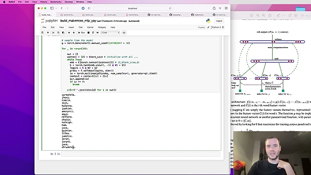
Sample names generated by the trained MLP character-level language model. [ 01:14:40 ]