Comprehensive Excel for Accounting: Mastering Formulas, PivotTables, Macros, and Charts
This video offers an in-depth guide to essential Excel skills for accounting professionals, covering efficient data handling and reporting.
- Keyboard Shortcuts [0:01:47]: Learn fundamental shortcuts like Ctrl + Arrow for navigation, Ctrl + 1 for formatting, Ctrl + Shift + 4 for currency, and Alt + = for SUM, significantly boosting efficiency.
- Number Formatting as Facade [0:11:52]: Understand that displayed formats (like currency, dates, percentages) can differ from the actual underlying numeric values, crucial for avoiding calculation errors. Ctrl + Shift + ` (tilde) reveals the raw number.
- Efficient Formula Creation [0:25:01]: Adhere to Excel's Golden Rule: use cell references for inputs that may change, and directly hard-code constants. Explore various formula types including calculating, logical (e.g.,
ISNUMBER[1:06:12]), and text formulas (e.g., joining first and last names [0:31:54]). - Lookup Formulas [0:49:50]: Master
VLOOKUPfor exact and approximate matches, and combineINDEXandMATCH[1:07:00] for powerful 2-way lookups and left-side data retrieval. - PivotTables for Dynamic Reporting [1:10:02]: Learn to create pivot tables from proper datasets, visualize reports, apply number formatting [1:17:44], pivot fields [1:21:21], change calculations (e.g., SUM to AVERAGE [1:22:42]), filter reports [1:25:55], group dates [1:33:42], and create linked pivot charts [1:39:00].
- Recorded Macros for Automation [1:51:05]: Automate repetitive tasks using the macro recorder, understanding the difference between absolute and relative references to handle static vs. variable report sizes.
- Chart Types & Best Practices [2:13:35]: Explore various chart types (column, bar, line, XY scatter), understand when to use each for effective data visualization, and learn formatting techniques like linking titles to cells [2:23:09].
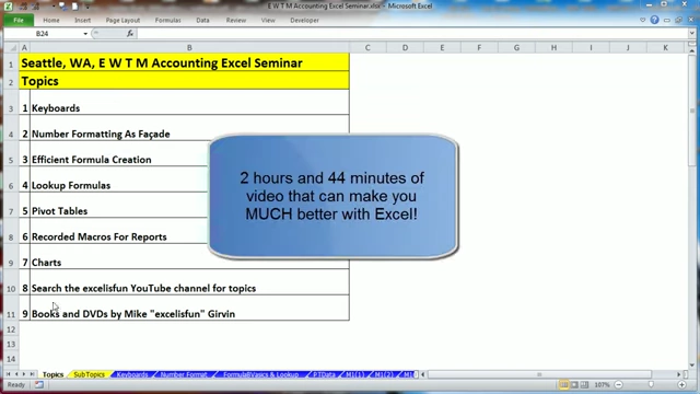
Video overview showing the table of contents of the training material [ 00:00:20 ]
Keyboards for Efficiency [0:01:47]
The video begins by emphasizing the importance of keyboard shortcuts for efficiency in Excel.
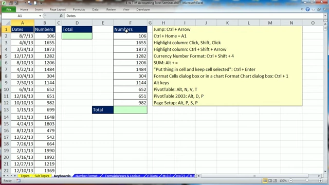
- Navigation and Selection:
Ctrl + Arrow[0:02:20]: Jumps to the edge of the current data region.Ctrl + Home[0:02:36]: Navigates to cell A1.Shift + Click[0:02:54]: Selects a range between the active cell and the clicked cell.Ctrl + Shift + Arrow[0:04:20]: Selects from the active cell to the end of the current data region in the direction of the arrow.
- Formatting Shortcuts:
- Ribbon and Quick Access Toolbar (QAT) Shortcuts:
- Function and Entry Shortcuts:
Alt + =[0:08:38]: Inserts theSUMfunction and attempts to guess the range.Shift + Enter[0:09:35]: Enters data into a cell and moves the active cell up.Ctrl + Enter[0:09:35]: Enters data into a cell and keeps the cell selected.Ctrl + Semicolon[0:14:12]: Enters today's hard-coded date.Ctrl + Shift + Semicolon[0:17:10]: Enters the current hard-coded time.Ctrl + Page Down[0:11:11]: Selects the next sheet to the right.Ctrl + Page Up[0:11:11]: Selects the next sheet to the left.
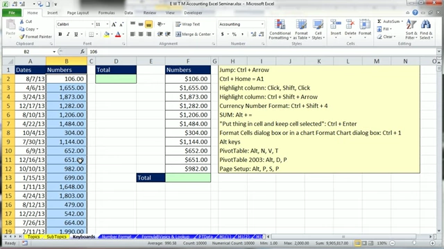
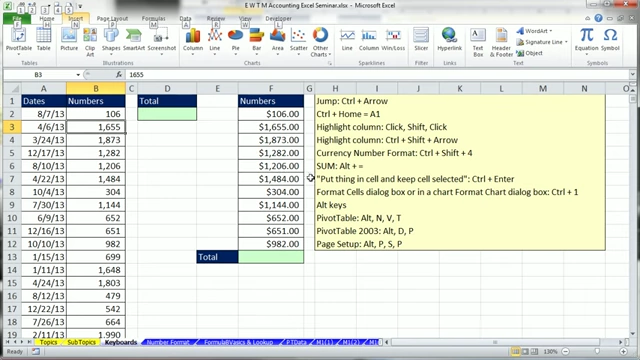
Number Formatting as Facade [0:11:52]
This section emphasizes a crucial concept: what is seen on the surface of a cell (the formatted number) is often different from what is actually stored in the cell.
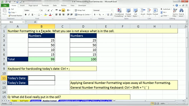
- Core Concept: Number formatting is like a facade or a mask. Formulas calculate based on the actual underlying number, not its display format.
- Example: Displaying "50" might hide "49.5" in the cell [0:13:10].
- Revealing Underlying Values:
Ctrl + Shift + Grave Accent(tilde) [0:14:58]: Applies the General number format, revealing the raw numeric value.
- Date Number Format [0:13:56]:
- Dates are stored as serial numbers, starting from January 1, 1900, as day 1.
- This allows for date arithmetic (e.g.,
Later_Date - Earlier_Dateto find days between dates [0:16:25]). - When calculating project days that include the start date, add
+1to the difference.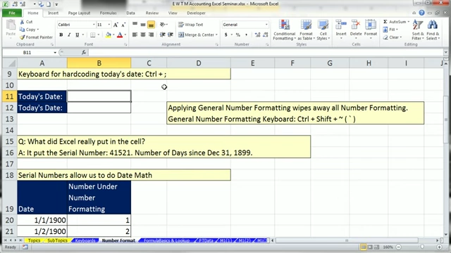
Excel showing the serial number representation of a date, illustrating the 'facade' concept [ 00:14:10 ]
- Time Number Format [0:17:10]:
- Time is stored as a decimal number between 0 and 1, representing the proportion of a 24-hour day (e.g., 8 AM is ~0.33, Noon is 0.5).
- To convert time differences into total hours (for payroll, for example), multiply the decimal result by 24 (e.g.,
(End_Time - Start_Time) * 24[0:20:25]).
- Percentage Number Format [0:21:25]:
- A common mistake is typing
3and then applying percentage format, resulting in300%. - Correct methods:
- Type
0.03then apply percentage format. - Pre-format the cell as percentage, then type
3(Excel interprets3as0.03when the cell is pre-formatted as percentage). - Type
3%directly into the cell (Excel stores0.03).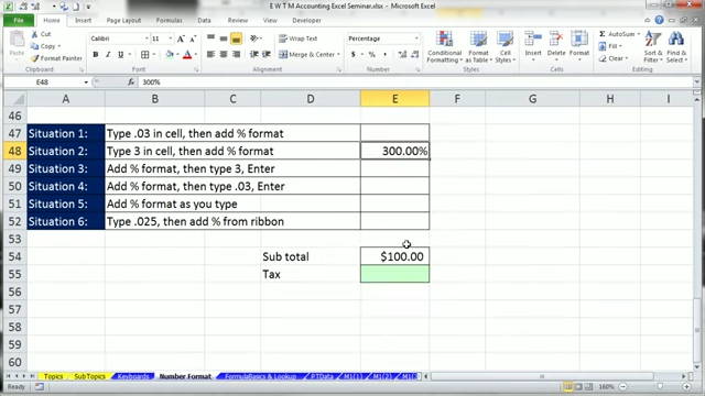
Different methods of typing percentages into Excel and their resulting formats [ 00:21:50 ]
- Type
- A common mistake is typing
Efficient Formula Creation [0:25:01]
The core principle for building robust and easy-to-manage spreadsheets.
- Excel's Golden Rule [0:25:01]: If a formula input (data, rates, parameters) can change, put it in a separate cell and refer to it using a cell reference in the formula. If it's a constant that will never change (like 12 months in a year), it's acceptable to hard-code it into the formula.
- Inefficient Formula Example (Tax Rate) [0:27:35]: Hard-coding
0.125directly makes the formula obscure and hard to update if the tax rate changes. - Efficient Formula Example (Tax Rate) [0:27:35]: Referencing a cell containing the tax rate (e.g.,
Amount * C25) makes the formula transparent and easily adaptable.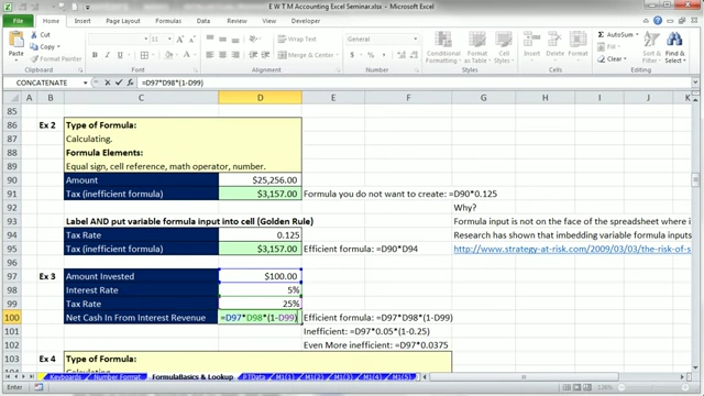
Comparison of inefficient (hard-coded) versus efficient (cell-referenced) formulas, illustrating Excel's Golden Rule [ 00:29:32 ]
- Inefficient Formula Example (Tax Rate) [0:27:35]: Hard-coding
- Formula Elements and Types:
- Calculating Formulas: Produce a numerical result (e.g.,
Revenue - SUM(Expenses)[0:30:00]). - Logical Formulas: Return
TRUEorFALSE(e.g.,C22 = D22to check if values are in balance [0:30:40]). Useful for identifying discrepancies in underlying values due to formatting. - Text Formulas: Combine text strings (e.g.,
First_Name & " " & Last_Name[0:31:54]). The ampersand (&) is the join symbol; spaces or other text must be enclosed in double quotes.
- Calculating Formulas: Produce a numerical result (e.g.,
- Functions with Criteria:
COUNTIF[0:33:29]: Counts cells based on a single criterion (e.g.,COUNTIF(Range, ">350")). When the criterion is a combination of an operator and a cell reference, use concatenation (e.g.,">" & C182[0:34:19]).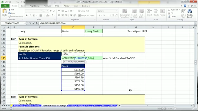
Using COUNTIF to count with criteria, showing the concatenation of an operator and a cell reference [ 00:34:03 ] SUMIFS[0:36:21]: Sums values based on one or more criteria. The sum range is specified first, followed by criteria ranges and their respective criteria.- Between Criteria for Dates/Numbers:
- For date ranges (e.g., sum between two dates): Use two criteria pairs with operators and dates (e.g.,
">=2013-09-20"and<="2013-10-09"[0:38:08]). Text dates are properly interpreted bySUMIFS. - For numeric ranges: Similar approach, defining lower and upper bounds with operators and numbers.
- For date ranges (e.g., sum between two dates): Use two criteria pairs with operators and dates (e.g.,
- Relative, Absolute, and Mixed Cell References [0:41:46]:
- Relative: Default behavior, references adjust when copied (e.g., A1 becomes A2, B1 etc.).
- Absolute (Locked): Achieved with
F4key (e.g.,$A$1), references do not change when copied. Used for constants like lookup tables. - Mixed: Locks either the row (
$A1) or the column (A$1). Crucial for efficiently copying formulas across a grid (e.g., budget calculations [0:43:58]), allowing a single formula to be copied across a 2D range.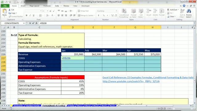
An Excel budget template demonstrating mixed cell references for efficient formula copying across a grid [ 00:48:50 ] - Using
Ctrl + Period[0:49:29] navigates between corners of a selected range, useful for checking formula references.
Lookup Formulas [0:49:50]
Formulas designed to retrieve specific data from a table based on a lookup value.
VLOOKUPFunction [0:49:50]:- Purpose: Looks for a value in the leftmost column of a table and returns a value in the same row from a specified column.
Vstands for vertical. - Arguments:
Lookup_value: The value to search for.Table_array: The range containing the lookup table. The first column must contain theLookup_value. This range should often be absolute.Col_index_num: The column number in theTable_arrayfrom which to retrieve the value.[Range_lookup]:FALSE(or0): Exact match (recommended for text or unsorted data).TRUE(or1, or omitted): Approximate match (for sorted numeric ranges like tax brackets).VLOOKUPwill find the largest value less than or equal to theLookup_value.
- Error Handling with
IFERROR[0:55:13]: WrapsVLOOKUPto display a custom message (e.g., "Not in List") or a blank cell ("") instead of#N/Aerrors when a match isn't found.
- Purpose: Looks for a value in the leftmost column of a table and returns a value in the same row from a specified column.
- Data Validation List [0:53:10]: Creates a dropdown list in a cell, allowing users to select from predefined options, ensuring accurate data entry and preventing lookup errors. Access via
Data > Data ValidationorAlt + D + L. - Comparing Two Lists [1:03:38]:
MATCHfunction: Returns the relative position of an item in a list (e.g.,MATCH("PCC", List, 0)returns2if "PCC" is the second item).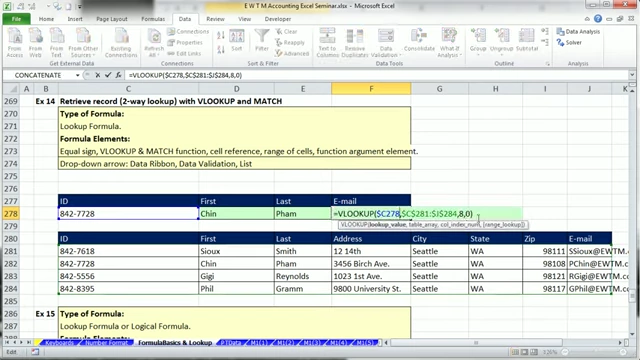
VLOOKUP function displaying its arguments, illustrating a 2-way lookup with MATCH for dynamic column selection [ 01:01:36 ] ISNUMBER(MATCH(...))[1:06:12]: ReturnsTRUEif an item is found in a list (i.e.,MATCHreturns a number),FALSEotherwise.ISNA(MATCH(...))[1:06:38]: ReturnsTRUEif an item is not found (i.e.,MATCHreturns#N/A),FALSEotherwise.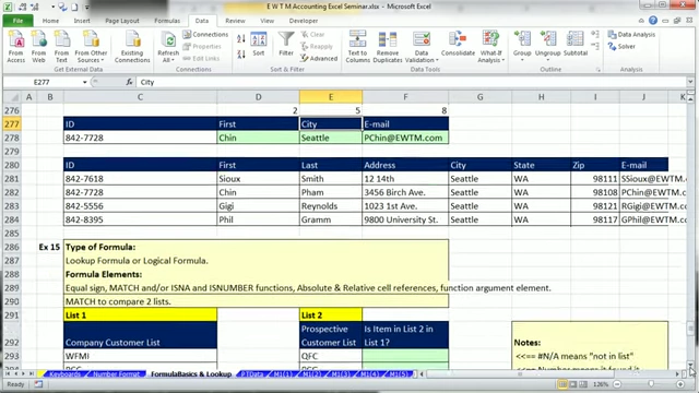
Comparing two lists in Excel to identify common or unique items using lookup functions [ 01:03:40 ]
INDEXandMATCHfor Left Lookup [1:07:00]:VLOOKUPcan only retrieve data to the right of the lookup column.INDEX(Return_Range, MATCH(Lookup_Value, Lookup_Column, 0))allows retrieving data from any column, including to the left.INDEXneeds a row number, andMATCHprovides this row number by finding the lookup value's position.
Pivot Tables [1:10:02]
Considered the most powerful feature in Excel for summarizing and analyzing large datasets.
- Proper Data Set [1:10:02]:
- Required structure: Field names (headers) at the top of each column, records in rows.
- Important: Data table should be surrounded by empty cells or the worksheet boundaries. Avoid notes or other data directly touching the main data table, as this can confuse Excel's automatic range detection.
- Avoid empty field names or entirely empty rows/columns within the data range.
- Creating a PivotTable [1:12:00]:
- Select any single cell within your data range.
- Go to
Insert > PivotTableor use the shortcutAlt + N + V + T[1:14:25]. - The dialog box typically guesses the range correctly. Choose to place it on a New Worksheet.
- Visualizing the Report [1:12:00]: Before dragging fields, mentally picture the desired output (e.g., regions as columns, sales reps as rows, units in values). This simplifies the drag-and-drop process.
- Dragging Fields [1:16:03]:
- Rows Area: For row headers/labels (e.g., Sales Rep, Product).
- Columns Area: For column headers/labels (e.g., Region).
- Values Area: For numerical data to be aggregated (e.g., Units, Sales). Defaults to SUM for numbers, COUNT for text/blanks.
- Filters Area: For overall report filtering (e.g., Customer).
- Report Layout & Design [1:16:58]:
- Change
Report LayouttoShow in Tabular Form[1:17:15] to display field names as column headers instead of "Row Labels". - Number Formatting [1:17:44]: Right-click any value in the pivot table, select
Value Field Settings > Number Format. This applies formatting directly to the field, so it persists even if the table is pivoted. - Custom Styles [1:19:05]: Create your own pivot table styles (e.g., for header rows, grand totals) via
Design > More (Styles) > New PivotTable Style.
- Change
- Pivoting the Report [1:21:21]: Drag fields between row, column, and filter areas to instantly rearrange the report's layout.
- Collapsing Rows [1:21:59]: If multiple fields are in the Rows area, use the
+/-buttons or right-clickExpand/Collapseto show/hide sub-levels. - Changing Calculation [1:22:42]: Right-click on a value in the pivot table, select
Summarize Values By, and choose from options likeSUM,COUNT,AVERAGE,MAX,MIN. - Filtering Options [1:24:46]:
- Field Filters: Use dropdown arrows on row/column labels for sorting, manual selection,
Label Filters(e.g., begins with "S"), orValue Filters(e.g., Top 10 items [1:25:25]). - Report Filters [1:25:55]: Drag a field to the Filters area. A dropdown appears above the pivot table to filter the entire report.
- Show Report Filter Pages [1:27:55]: A powerful feature under
Options > Options > Show Report Filter Pages. For each item in a report filter, it creates a separate worksheet with the pivot table filtered for that item (e.g., 20 customers result in 20 separate worksheets). - Slicers [1:28:30]: A more user-friendly visual filter (introduced in Excel 2010). Insert via
Options > Insert Slicer. Allows single or multi-selection with visual feedback.
- Field Filters: Use dropdown arrows on row/column labels for sorting, manual selection,
- Formulas vs. PivotTables [1:30:13]:
- PivotTables are Easy: Quick to create complex summaries.
- Formulas are Flexible: Offer nearly infinite calculation possibilities (pivot tables have limited aggregate functions).
- Formulas Update Instantly: Pivot tables require manual refresh (
Right-Click > Refresh[1:32:46]) when source data changes.
- Grouping in PivotTables:
- Grouping Dates [1:33:42]: Right-click on a date field in the pivot table and select
Group. Can group byMonths,Quarters,Years, etc. - Grouping Numbers [1:35:41]: Right-click on a numeric field and select
Group. DefineStarting at,Ending at, andBy(increment size). Labels differ for integers vs. decimals. - Troubleshooting Grouping: If grouping dates fails, it's often due to empty cells or dates stored as text in the source data.
- Grouping Dates [1:33:42]: Right-click on a date field in the pivot table and select
- Pivot Charts [1:39:00]:
- One-click creation from a pivot table (
Options > PivotChart). - Dynamically linked: Filtering or pivoting the pivot table will update the chart automatically.
- One-click creation from a pivot table (
- Advanced Value Calculations (
Show Values As) [1:40:45]: - Multiple Calculations in One PivotTable [1:46:26]: Drag the same value field multiple times to the Values area, and then change each instance's summary function (e.g., Sum, Average, Count).
- Handling Empty Cells and Data Types:
- Multiple PivotTables and Data Cache: By default (since Excel 2007), new pivot tables from the same data source use the same in-memory cache, meaning grouping changes apply to all. To create a pivot table with a separate cache, use the legacy PivotTable and PivotChart Wizard (
Alt + D + P[1:47:54]).
Recorded Macros for Reports [1:51:05]
Macros automate repetitive tasks by recording user actions as VBA (Visual Basic for Applications) code.
- Enabling Macros:
- Show
Developertab:Right-click Ribbon > Customize Ribbon > Check Developer. - Save workbook as
.xlsm(Macro-Enabled Workbook) [1:52:39] (File > Save As > .xlsm). - Macro Security: Set to
Disable all macros with notificationfor safety.
- Show
- Recording Basics:
- Click
Record Macroon the Developer tab. - Give it a descriptive name (no spaces) and optionally assign a shortcut key (e.g.,
Ctrl + Shift + F). - Choose where to store the macro:
This Workbook(for current file only) orPersonal Macro Workbook(hidden workbook, accessible universally on your computer) [1:55:10]. - Perform the steps you want to automate.
- Click
Stop Recording.
- Click
- Absolute vs. Relative References in Macros:
- Absolute (Default): Records exact cell addresses (e.g.,
Range("A1").Select). Suitable for reports that are always in the same location and size (Format Static Report[1:55:36]). - Relative: Records movements relative to the active cell (e.g.,
ActiveCell.Offset(1, 0).Select). Essential for reports with variable height/width (Format Report Variable Height[2:04:07]). ToggleUse Relative Referenceson/off during recording as needed.- Trick for Variable Height Reports [2:00:51]: Use
Ctrl + Arrowto jump to the end of data ranges, as this action records a relative movement (Selection.End(xlDown).Select), adapting to different data sizes. - Trick for Pasting Formulas [2:05:43]: After entering a formula, use relative selection (
ActiveCell.Offset(...)) and thenCtrl + Shift + Up Arrowto select the variable range for auto-filling.
- Trick for Variable Height Reports [2:00:51]: Use
- Absolute (Default): Records exact cell addresses (e.g.,
- Rearranging Records (Transpose) [2:09:01]: A macro can copy a vertical block of data and paste it horizontally (
Paste Special > Transpose), then delete the original vertical data. This is a powerful application of relative references for data transformation.- Important: Always start the macro in a specific, repeatable location relative to the data to be processed.
Charts [2:13:35]
Visual tools for presenting data.
- Chart Types [2:13:35]:
- Pie Charts [2:14:05]: Best for comparing parts to a whole (percentages). Avoid 3D or exploded pies (chart junk) as they distort perception.
- Column Charts [2:15:05]: Vertical bars comparing values across categories.
- Bar Charts [2:15:30]: Horizontal bars, similar to column charts, sometimes better for emphasizing differences or if categories have long names.
- Stacked Column/Bar Charts [2:15:58]: Show components of a total within each category.
- Line Charts [2:16:28]: Show trends over categories (e.g., time). One data series (Y-value) per point on X-axis, X-axis categories are equidistant.
- XY Scatter Charts [2:16:37]: Show the relationship between two numerical variables (X and Y). Use dots for sampled/collected data (e.g., study hours vs. test scores [2:37:09]), and lines for models or continuous predictions (e.g., break-even analysis [2:41:28]).
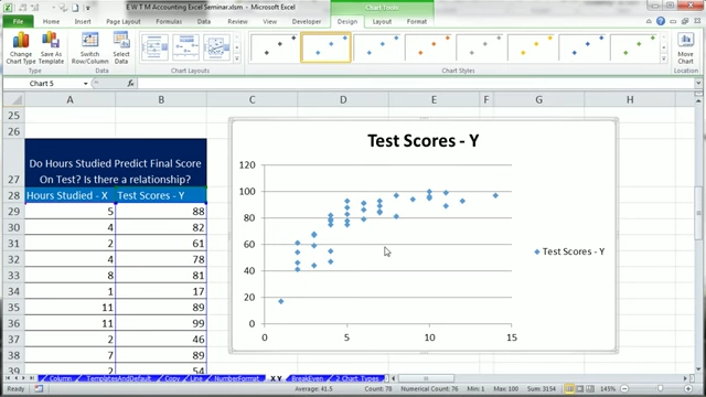
An XY Scatter chart showing the relationship between 'Hours Studied' and 'Test Scores' [ 02:38:31 ] - Histograms (Column charts with no gaps) [2:17:35]: Used for frequency distributions where categories represent continuous numerical bins.
- Creating Charts:
- Chart Interpretation by Excel: Excel tries to guess which data goes to axis labels and which to series based on the number of rows vs. columns.
- Formatting Charts:
- Linking Chart Titles to Cells [2:23:09]: Select the chart title, type
=in the formula bar, and click the cell containing the desired title text. This links the title, so it updates automatically. - Formatting Chart Elements: Select any chart element (axis, legend, data series) and press
Ctrl + 1to open its specific Format dialog box. - Custom Number Formatting on Axes [2:34:52]: Use custom number formats (e.g.,
#,,"K"for thousands [2:35:05]) to display large numbers concisely on axes.
- Linking Chart Titles to Cells [2:23:09]: Select the chart title, type
- Saving Chart Templates [2:25:43]:
- Format a chart to your preference.
Design > Save as Template. Give it a name.- To use:
Insert > Other Charts > All Chart Types > Templates.
- Setting Default Chart [2:26:48]:
- After saving a template, right-click the template in the
Insert Chartdialog and selectSet as Default Chart. This makesAlt + F1create this specific chart type/style.
- After saving a template, right-click the template in the
- Copying Charts [2:27:45]: Click the outer border of the chart (not an internal element) and
Ctrl + C. ThenCtrl + Vto paste. - Changing Chart Type for a Series [2:43:39]: Right-click on a data series (e.g., the bars representing expenses) and choose
Change Series Chart Typeto convert just that series to a different type (e.g., a line chart overlaid on column charts). This creates powerful combined charts.